Insights
How to Build a Three Statement Model (Update)
I recorded the first video for this website in 2013 with a $27 microphone I purchased at Best Buy. Since that time, the technology and software used at ASM has improved significantly, and I thought it was time to update the original recording.
Monthly Debt Schedules Example
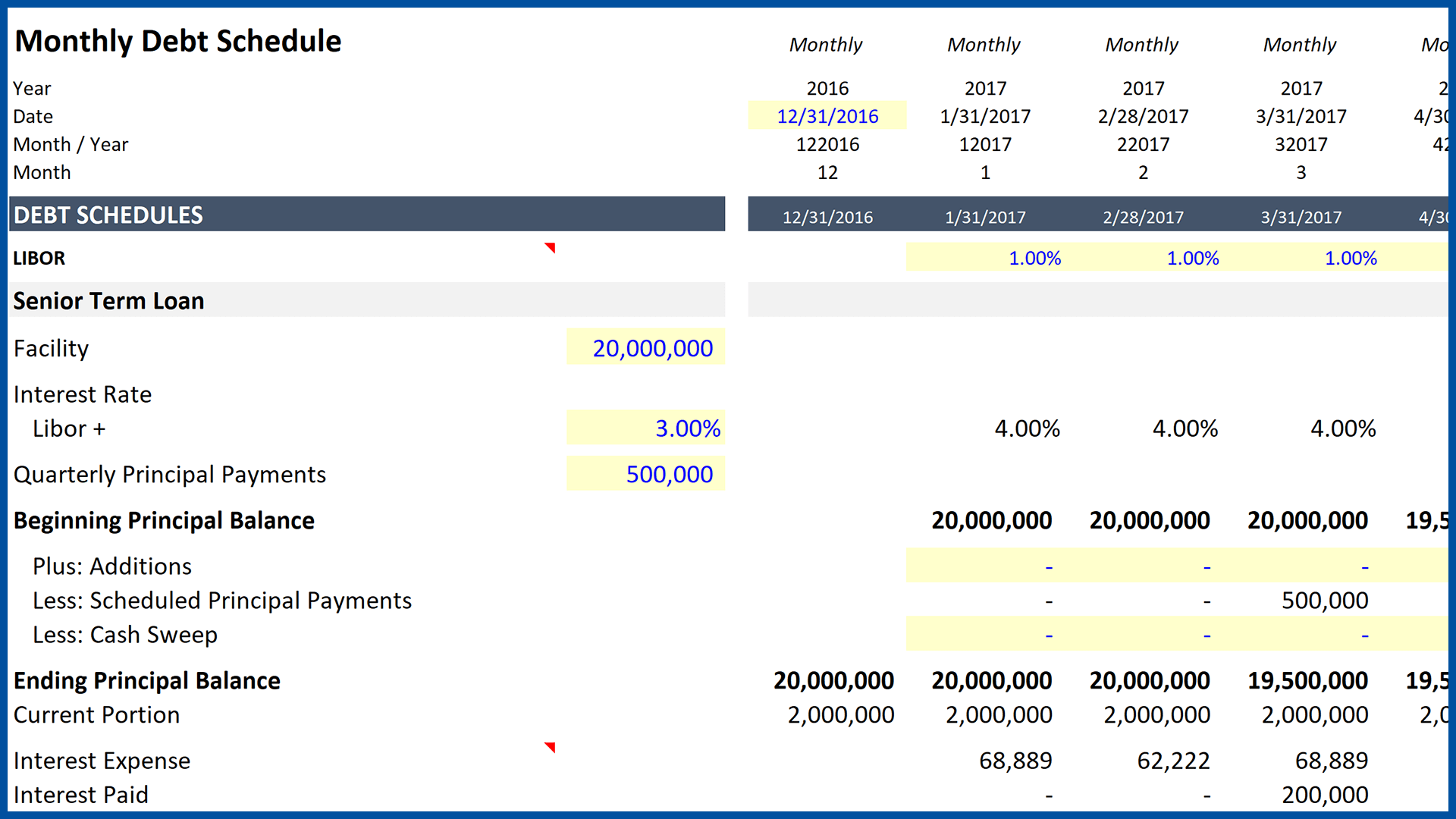
This post includes an Excel template with two examples (available for download at the bottom of this post). The first it labeled “Senior Term Loan,” and the second is labeled “Subordinated Notes.”
Excel: =MOD() to Calculate Quarterly Interest Payments
One of the challenges you will encounter building monthly debt schedules is the need to calculate and show interest expense in each month, and then reflect the payment of interest at the end of the quarter. This video provides a helpful approach.
Excel Trick: Sum a Specific Number of Cells
This video explains how the =SUM and =OFFSET functions can be combined to write a formula that will sum a specific number of cells. This is especially useful when you are working with monthly data, and showing quarterly and annual periods in a financial model. The video also explains why using the =SUM formula for this purpose can lead to errors.
Independent Sponsor Economics
Before discussing the economics, I thought a definition of a fundless sponsor would be helpful. An article in The Economist provided an excellent example: “The typical search-fund principals are MBA graduates from an elite American university, who raise $400,000 or so of “walking around money” from investors, who purchase a stake in the fund for about $40,000 a share. The fund searches for a high-growth, high-margin target, valued at $5m-20m. The fledgling businessmen then hold a second round of acquisition financing, as well as raising debt. Their tenure as bosses lasts until they sell out.” [1]