In this video we are going to learn how to use the =INDIRECT function to create flexible inputs for Excel Table formulas. An indirect structured table reference will allow us to quickly evaluate data sets based on different fields.
For example, in the image below, the field being summed can be changed with the value in cell B17 (circled red in the image). Cell D17 contains an INDEX+MATCH formula that returns the field based on the number next to it. If you were to input a value of 1 in cell B17, for example, the formula in cell D17 would return “No. of Shipments,” and the formula in cell D21 would return the sum of all values in the “No. of Shipments” column.

The =INDIRECT function works by turning text into a cell reference. By way of example, the formula in D21 is using the =INDIRECT function to mirror the formula in D27. In the image above, the values in cells D21 and D27 would be identical.
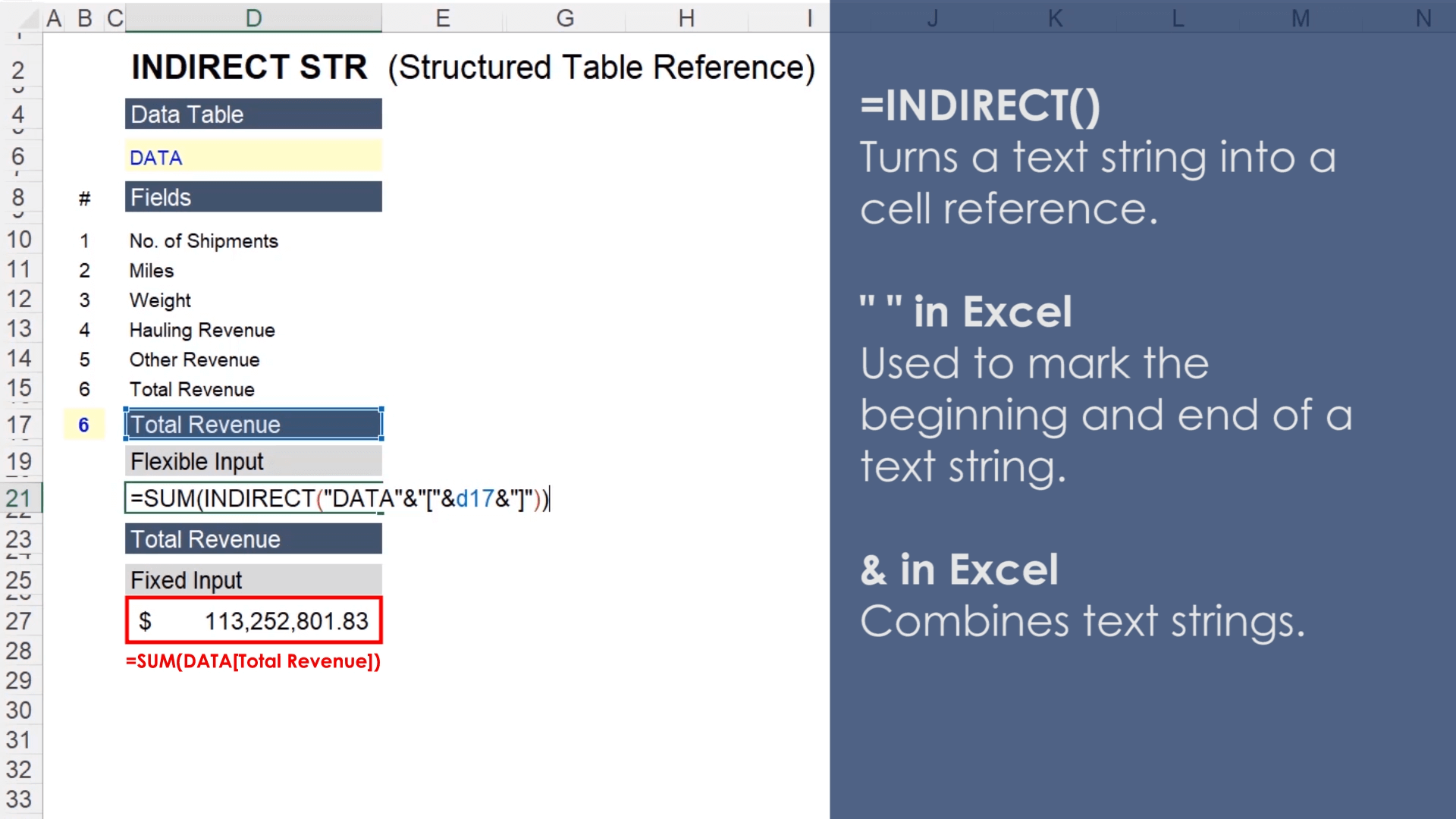
With that in mind, let’s explore the ampersand operator in Excel to better understand the formula in cell D21. In Excel, the ampersand (&) is used to combine text strings and quotation marks are used to denote the beginning and end of a text string. So Excel interprets the text inside the INDIRECT Function in cell D21 as “DATA[Total Revenue].”
This may seem simple, but it creates substantially more flexibility in the formulas we will use to analyze our data set. Please see the video for more detail.