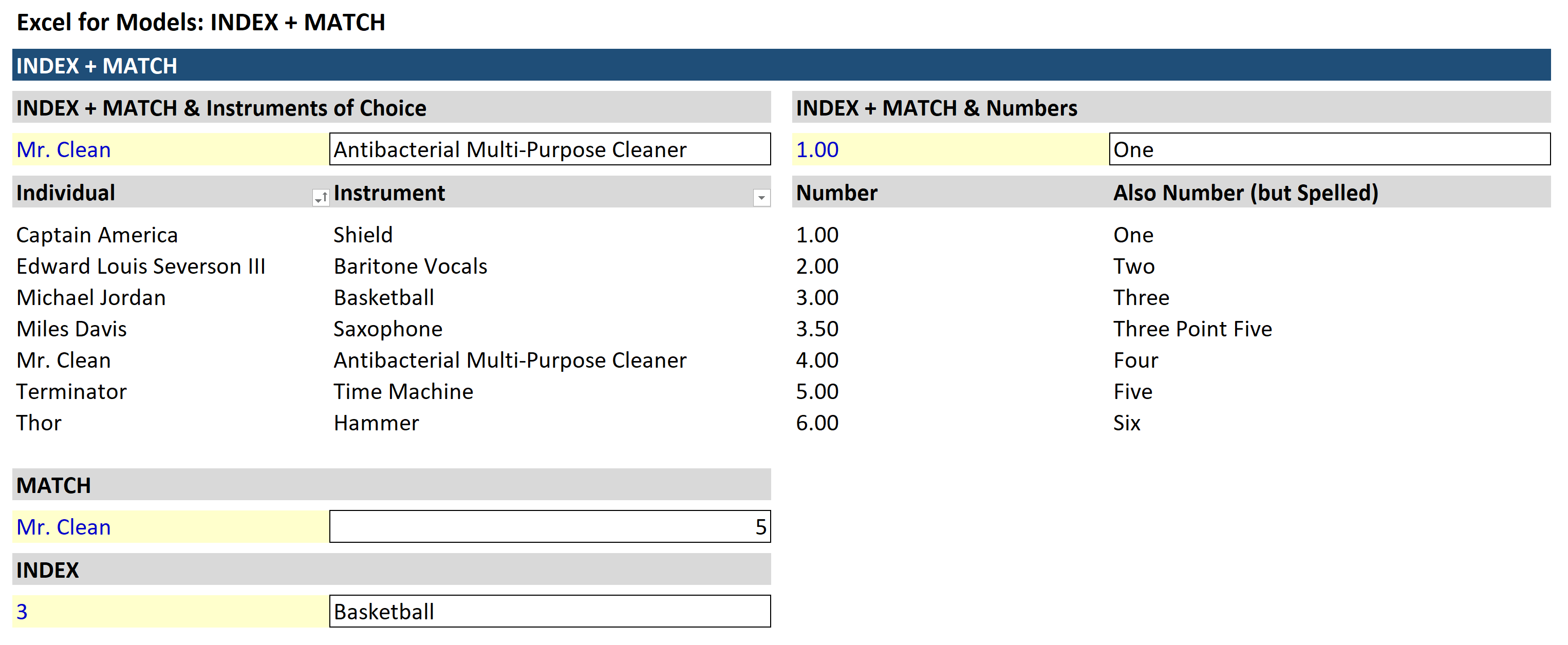
In Excel, the INDEX and MATCH functions can be combined to create a very useful lookup function. To demonstrate how this works, this video will first explain how MATCH returns a location based on an input, and then explain how INDEX uses that location to return the desired value. (Please refer to the first image available below to see the values returned by the formulas and functions that follow.)

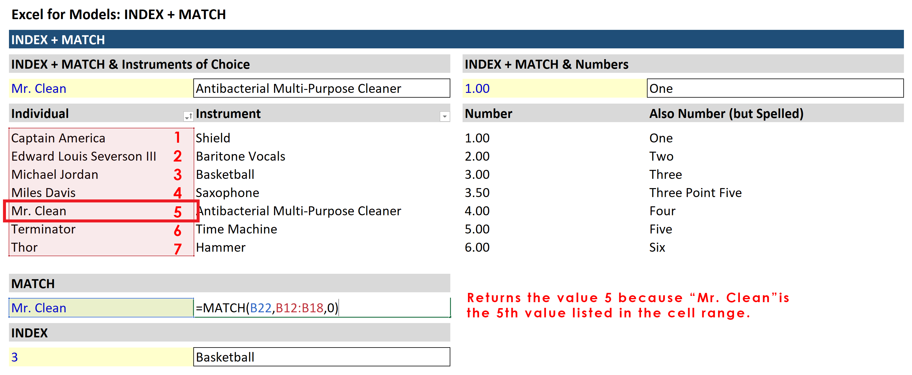
Per the image below, the MATCH function is looking for the value "Mr. Clean" in the cell range B12:B18. It returns a value of 5 because "Mr. Clean" is the 5th value listed in the cell range.

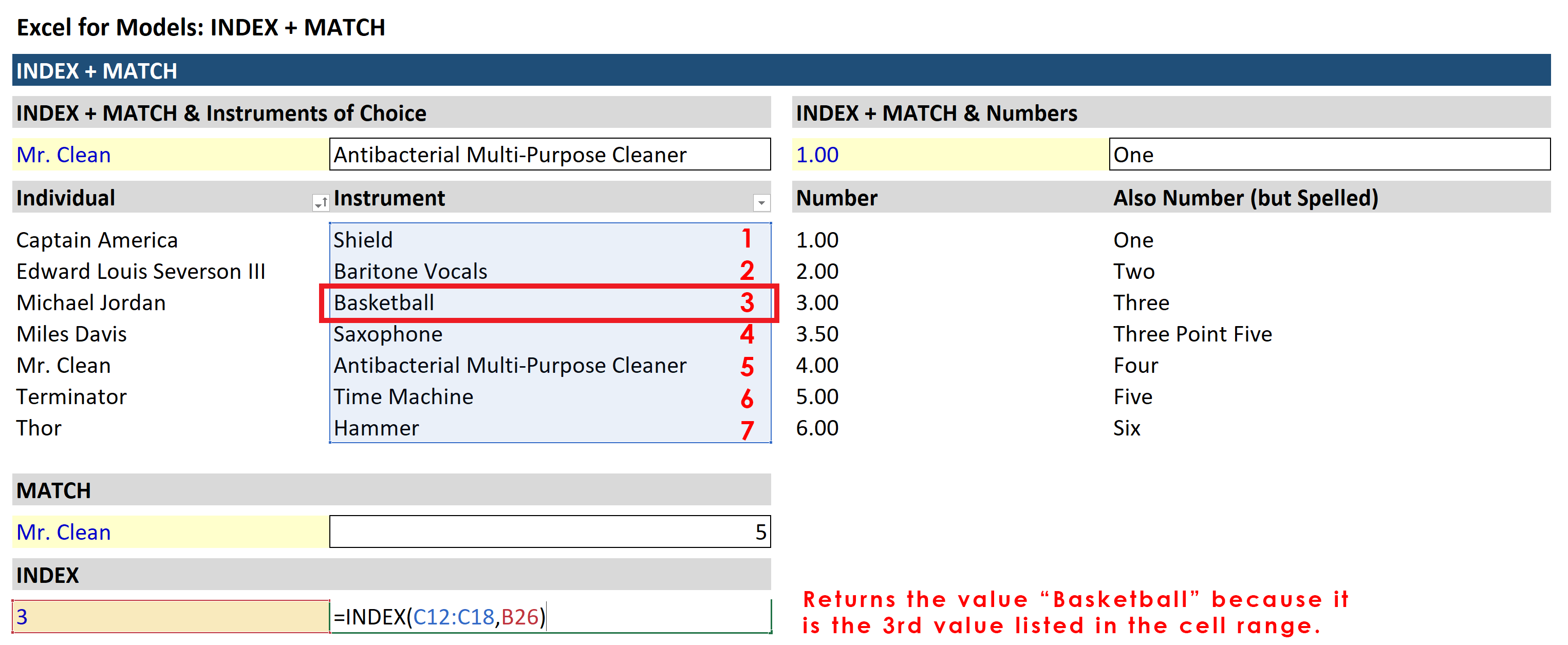
INDEX returns the value based on the location provided. In the example provided below, you will see that INDEX returns the value "Basketball" because it is the 3rd value listed in the cell range.

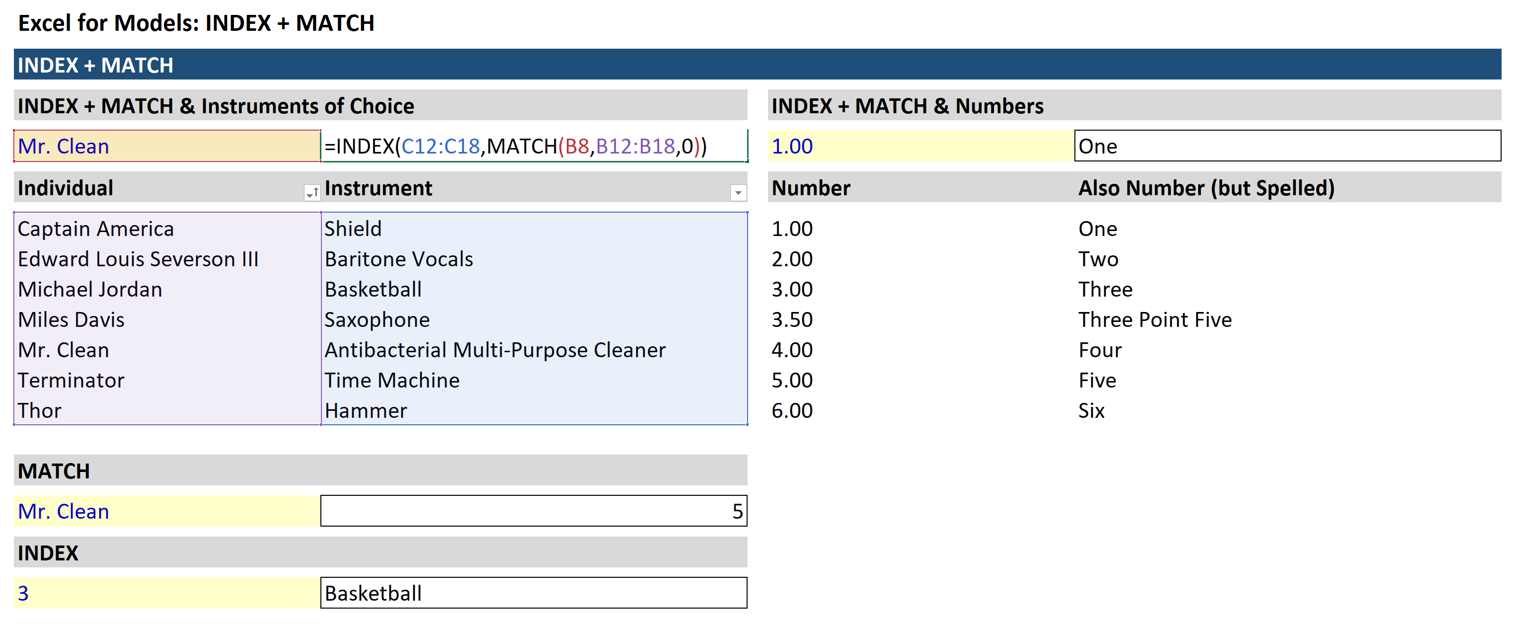
In the last image you will see how these two functions combine. Starting with the embedded MATCH function, which will return a value of 5 as it looks for "Mr. Clean" in the cell range B12:B18. The INDEX function then takes this value of 5 and applies it to the adjacent array in blue (C12:C18). The 5th value in the cell range C12:C18 is "Antibacterial Multi-Purpose Cleaner," which is the value you will see in the first image above.

Please see the video for more instruction.